Solving Nonlinear Equations
Learning objectives
- Evaluate the bisection, newton, and secant methods to solve nonlinear equations in 1D
- Apply Newton's method to solve a nonlinear system of equations
Root of a Function
Consider a function \(f : \mathbb{R} \to \mathbb{R}\). The point \(x \in \mathbb{R}\) is called the root of \(f\) if \(f(x) = 0\).
Solution of an Equation
Finding the values of \(x\) for which \(f(x) = 0\) is useful for many applications, but a more general task is to find the values of \(x\) for which \(f(x) = y\). The same techniques used to find the root of a function can be used to solve an equation by manipulating the function like so:
\[\tilde{f}(x) = f(x) - y = 0\]The new function \(\tilde{f}(x)\) has a root at the solution to the original equation \(f(x) = y\).
Nonlinear Equations in 1D
Linear functions are trivial to solve, as are quadratic functions if you have the quadratic formula memorized. However, polynomials of higher degree and non-polynomial functions are much more difficult to solve. The simplest technique for solving these types of equations is to use an iterative root-finding technique. Instead of finding out where \(f(x) = 0\) directly, we will start with an initial guess and improve it over multiple steps until our residual \(f(x)\) is sufficiently small.
Convergence
An iterative method converges with rate \(\mathbf r\) if:
\[\lim_{k\to\infty} \frac{\|e_{k + 1}\|}{\|e_{k}\|^{\mathbf r}} = C, \quad 0 < C < \infty\]where \(e_k\) is the error at iteration k.
\[\begin{eqnarray} \mathbf{r} &=& 1: linear\ convergence\\ \\ 1 < \mathbf{r} &<& 2: superlinear\ convergence\\ \\ \mathbf{r} &=& 2: quadratic\ convergence\\ \end{eqnarray}\]Linear convergence gains a constant number of accurate digits each step (the error shrinks linearly). When \(C\) is close to 1 convergence is slow.
Quadratic convergence doubles the number of accurate digits in each step (the error shrinks quadratically). However it only starts making sense once \(\|e^k\|\) is small, and C does not matter much.
Example
What is the convergence rate of Power Iteration?
Answer
Recall from the power iteration method
\[\lim_{k\to\infty} \frac{\|e_{k + 1}\|}{\|e_{k}\|^{\mathbf 1}} = |\frac{\lambda_{2}} {\lambda_{1}}| = C\]We see that when \({\mathbf r} = 1\), we get a constant for the ratio between two consecutive iterations. Therefore power iteration has linear convergence.
Bisection Method
The bisection method is the simplest root-finding technique.
Algorithm
The algorithm for bisection is analogous to binary search:
- Take two points, \(a\) and \(b\), on each side of the root such that \(f(a)\) and \(f(b)\) have opposite signs.
- Calculate the midpoint \(c = \frac{a + b}{2}\)
- Evaluate \(f(c)\) and use \(c\) to replace either \(a\) or \(b\), keeping the signs of the endpoints opposite.
With this algorithm we successively half the length of the interval known to contain the root each time. We can repeat this process until the length of the interval is less than the tolerance to which we want to know the root.
Convergence
The bisection method does not estimate \(x_{k}\), the approximation of the desired root \(x\). It instead finds an interval (smaller than a given tolerance), that contains the root.
Therefore, the error at iteration k is defined to be the length of the interval at k iterations or \(\frac{(b - a)}{2^k}\).
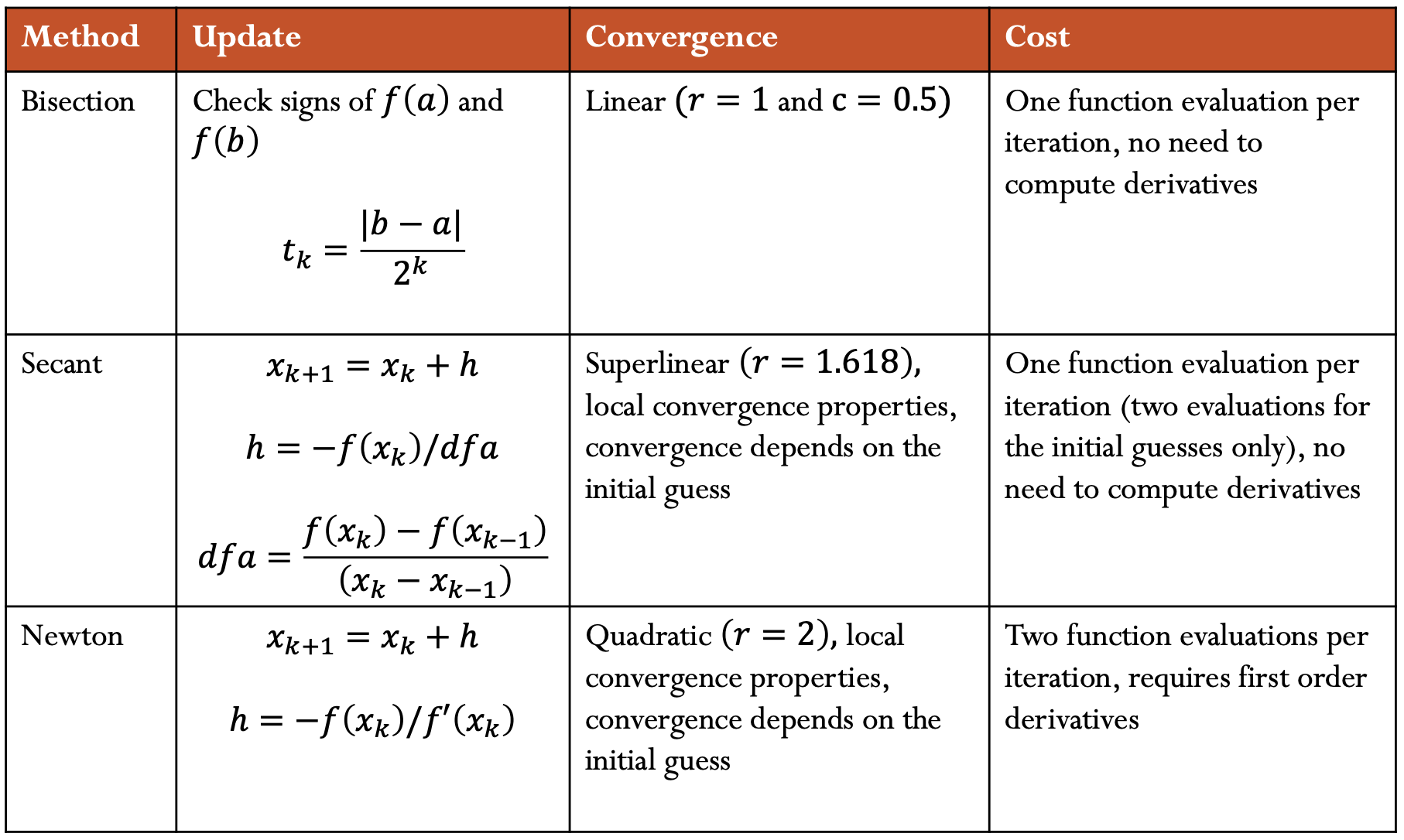
\[\lim_{k\to\infty} \frac{\|e_{k + 1}\|}{\|e_{k}\|^{\mathbf r}} = \lim_{k\to\infty} \frac{\|\frac{(b - a)}{2^{k + 1}}\|}{\|\frac{(b - a)}{2^k}\|} = 0.5\]Which gives us linear convergence, with a constant of \(\frac{1}{2}\).
Computational Cost
Conceptually bisection method uses 2 function evaluations at each iteration. However, at each step either one of \(a\) or \(b\) stays the same. So, at each iteration (after the first iteration), one of \(f(a)\) or \(f(b)\) was computed during the previous iteration. Therefore, bisection method requires only one new function evaluation per iteration. Depending on how costly the function is to evaluate, this can be a significant cost savings.
Drawbacks
The bisection method requires us to know a little about our function. Specifically, \(f(x)\) must be continuous and we must have an interval \([a, b]\) such that
\[\mathrm{sgn}(f(a)) = -\mathrm{sgn}(f(b)).\]Then, by the intermediate value theorem, we know that there must be a root in the interval \([a,b]\).
This restriction means that the bisection method cannot solve for the root of \(x^2\), as it never crosses the x-axis and becomes negative.
Example
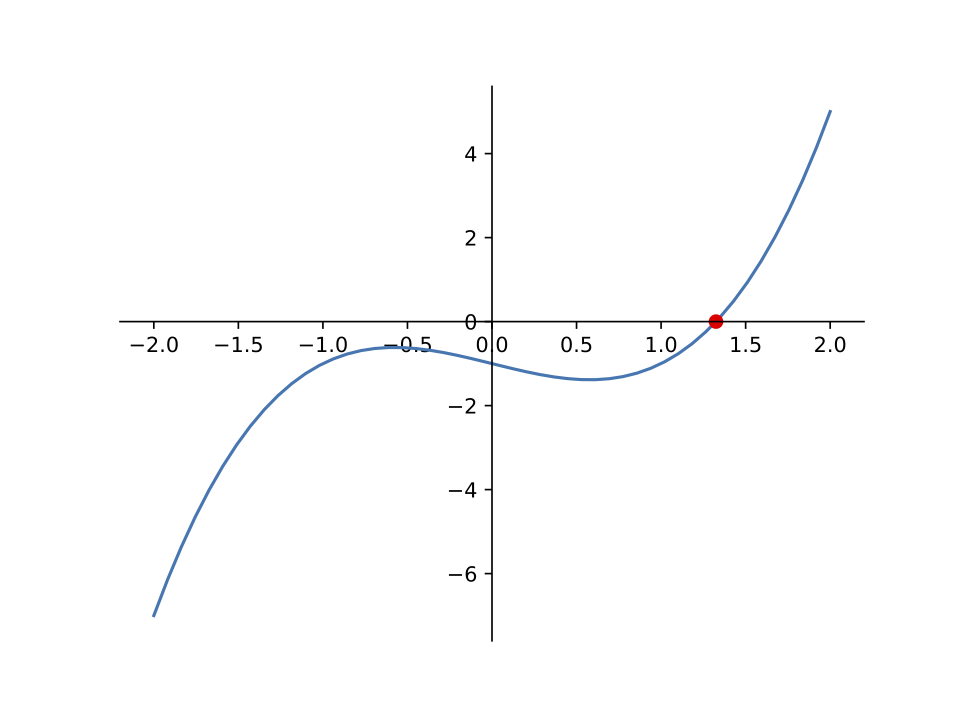
\[f(x) = x^3 - x - 1\]Answer

From the graph above, we can see that \(f(x)\) has a root somewhere between 1 and 2. It is difficult to tell exactly what the root is, but we can use the bisection method to approximate it. Specifically, we can set \(a = 1\) and \(b = 2\).
Iteration 1
Since \(f(b)\) and \(f(c)\) are both positive, we will replace \(b\) with \(c\) and further narrow our interval.
Iteration 2
Since \(f(a)\) and \(f(c)\) are both negative, we will replace \(a\) with \(c\) and further narrow our interval.
Note that as described above, we didn't need to recalculate \(f(a)\) or \(f(b)\) as we had already calculated them during the previous iteration. Reusing these values can be a significant cost savings.
Iteration 3
Since \(f(b)\) and \(f(c)\) are both positive, we will replace \(b\) with \(c\) and further narrow our interval.
…
Iteration n
When running the code for bisection method given below, the resulting approximate root determined is \(1.324717957244502\). With bisection, we can approximate the root to a desired tolerance (the value above is for the default tolerances).
Code
The following Python code calls SciPy's bisect method:
import scipy.optimize as opt

def f(x):
    return x**3 - x - 1

root = opt.bisect(f, a=1, b=2)
Newton's Method
The Newton-Raphson Method (a.k.a. Newton's Method) uses a Taylor series approximation of the function to find an approximate solution. Specifically, it takes the first 2 terms:
\[f(x_k + h) \approx f(x_k) + f'(x_k)h\]Algorithm
Starting with the Taylor series above, we can find the root of this new function like so:
\[f(x_k) + f'(x_k)h = 0\] \[h = - \frac{f(x_k)}{f'(x_k)}\]This value of \(h\) is known as the Newton step. Now, \(h\) can be used to perform a Newton update, to find a value of \(x\) closer to the root of \(f\):
\[\begin{eqnarray} x_{k+1} &=& x_k + h \\ &=& x_k - \frac{f(x_k)}{f'(x_k)} \end{eqnarray}\]Geometrically, \((x_{k+1}, 0)\) is the intersection of the x-axis and the tangent of the graph at \((x_k, f(x_k))\).
By repeating this procedure, we can get closer and closer to the actual root.
Computational Cost
With Newton's method, at each iteration we must evaluate both \(f(x)\) and \(f'(x)\).
Convergence
Although Newton's method is more costly than the bisection method, it converges quicker.
\[\lim_{k\to\infty} \frac{\|e_{k + 1}\|}{\|e_{k}\|^{\mathbf 2}} = C\]Which gives us quadratic convergence. However, as we see in the next section, this can depend on the initial guess.
Drawbacks
The additional cost of evaluating the derivative makes each iteration slower to compute.
Many functions are not easily differentiable, so Newton's Method is not always possible. Even in cases when it is possible to evaluate the derivative, it may be quite costly.
Convergence only works well if you are already close to the root. Specifically, if started too far from the root Newton's method may not converge at all.
Example
\[\begin{align*} f(x) &= x^3 - x - 1 \\ f'(x) &= 3x^2 - 1 \end{align*}\]Answer

From the graph above, we can see that the root is somewhere near \(x = 1\). We will use \(x_0\) as our starting position.
Iteration 1
\(\begin{flalign*} \hspace{2cm} x_1 &= x_0 - \frac{f(x_0)}{f'(x_0)} \\ &= 1 - \frac{f(1)}{f'(1)} &\\ &= 1 - \frac{1^3 - 1 - 1}{3 \cdot 1^2 - 1} \\ &= 1 + \frac{1}{2} \\ &= 1.5 \end{flalign*}\)
Iteration 2
\(\begin{flalign*} \hspace{2cm} x_2 &= x_1 - \frac{f(x_1)}{f'(x_1)} \\ &= 1.5 - \frac{f(1.5)}{f'(1.5)} &\\ &= 1.5 - \frac{1.5^3 - 1.5 - 1}{3 \cdot 1.5^2 - 1} \\ &= 1.5 - \frac{0.875}{5.75} \\ &= 1.3478260869565217 \end{flalign*}\)
Iteration 3
As you can see, Newton's Method is already converging significantly faster than the Bisection Method.
…
Iteration n
When running the code for Newton's method given below, the resulting approximate root determined is \(1.324717957244746\).
Code
The following Python code calls SciPy's newton method:
import scipy.optimize as opt

def f(x):
    return x**3 - x - 1

def fprime(x):
    return 3 * x**2 - 1

root = opt.newton(f, x0=1, fprime=fprime)
Secant Method
Like Newton's Method, secant method uses the Taylor Series to find the solution. However, you may not always be able to take the derivative of a function. Secant method gets around this by approximating the derivative as:
\[f'(x_k) \approx \frac{f(x_k) - f(x_{k-1})}{x_k - x_{k-1}}\]Algorithm
The steps involved in the Secant Method are identical to those of the Newton Method, with the derivative replaced by an approximation for the slope of the tangent.
Computational Cost
Similar to bisection, although secant method conceptually requires 2 function evaluations per iteration, one of the function evaluations will have been computed in the previous iteration and can be reused. So, secant method requires 1 new function evaluation per iteration (after the first iteration).
Convergence
Secant method has superlinear convergence.
More specifically, the rate of convergence \(r\) is:
\[r = \frac{1 + \sqrt{5}}{2} \approx 1.618\]This happens to be the golden ratio.
Drawbacks
This technique has many of the same drawbacks as Newton's Method, but does not require a derivative. It does not converge as quickly as Newton's Method. It also requires two starting guesses near the root.
Example
\[f(x) = x^3 - x - 1\]Answer

Let's start with \(x_0 = 1\) and \(x_{-1} = 2\).
Iteration 1
First, find an approximate for the derivative (slope):
Then, use this for Newton's Method:
\(\begin{flalign*} \hspace{0.5cm}x_1 &= x_0 - \frac{f(x_0)}{f'(x_0)} \\ &= 1 - \frac{f(1)}{f'(1)} &\\ &= 1 - \frac{1^3 - 1 - 1}{6} \\ &= 1 + \frac{1}{6} \\ &= 1.1666666666666667 \end{flalign*}\)
Iteration 2
\(\begin{flalign*} \hspace{0.5cm}x_2 &= x_1 - \frac{f(x_1)}{f'(x_1)} \\ &= 1.1666666666666667 - \frac{f(1.1666666666666667)}{f'(1.1666666666666667)} &\\ &= 1.1666666666666667 - \frac{1.1666666666666667^3 - 1.1666666666666667 - 1}{2.5277777777777777} \\ &= 1.1666666666666667 - \frac{-0.5787037037037035}{2.5277777777777777} \\ &= 1.3956043956043955 \end{flalign*}\)
Iteration 3
…
Iteration n
When running the code for secant method given below, the resulting approximate root determined is \(1.324717957244753\).
Code
SciPy's newton method serves double-duty. If given a function \(f\) and a first derivative \(f'\), it will use Newton's Method. If it is not given a derivative, it will instead use the Secant Method to approximate it:
import scipy.optimize as opt

def f(x):
    return x**3 - x - 1

root = opt.newton(f, x0=1)
1D Summary

Nonlinear System of Equations
Similar to root-finding in 1 dimension, we can also perform root-finding for multiple equations in \(n\) dimensions. Mathematically, we are trying to solve \(\boldsymbol{f(x) = 0}\) for \(\boldsymbol{f} : \mathbb{R}^n \to \mathbb{R}^n\). In other words, \(\boldsymbol{f(x)}\) is now a vector-valued function
\[\boldsymbol{f(x)} = \begin{bmatrix} f_1(\boldsymbol{x}) \\ \vdots \\ f_n(\boldsymbol{x}) \end{bmatrix} = \begin{bmatrix} f_1(x_1, \ldots, x_n) \\ \vdots \\ f_n(x_1, \ldots, x_n) \end{bmatrix}\]If we are instead looking for the solution to \(\boldsymbol{f(x) = y}\), we can rework our function like so:
\[\boldsymbol{\tilde{f}(x)} = \boldsymbol{f(x)} - \boldsymbol{y} = \boldsymbol{0}\]We can think of each equation as a function that describes a surface. We are looking for vectors that describe the intersection of these surfaces.
The Jacobian Matrix
Given \(\boldsymbol{f} : \mathbb{R}^n \to \mathbb{R}^n\) we define the Jacobian matrix \({\bf J}_f\) as:
\[{\bf J}_f(\boldsymbol{x}) = \begin{bmatrix} \frac{\partial f_1}{\partial x_1} & \ldots & \frac{\partial f_1}{\partial x_n} \\ \vdots & \ddots & \vdots \\ \frac{\partial f_n}{\partial x_1} & \ldots & \frac{\partial f_n}{\partial x_n} \end{bmatrix}\]Newton's Method
The multi-dimensional equivalent of Newton's Method involves approximating a function as:
\[\boldsymbol{f(x + s)} \approx \boldsymbol{f(x)} + {\bf J}_f(\boldsymbol{x})\boldsymbol{s}\]where \({\bf J}_f\) is the Jacobian matrix of \(\boldsymbol{f}\).
By setting this to \(\mathbf{0}\) and rearranging, we get:
\[\begin{align*} {\bf J}_f(\boldsymbol{x})\boldsymbol{s} &= -\boldsymbol{f(x)} \qquad \qquad (1) \\ \boldsymbol{s} &= - {\bf J}_f(\boldsymbol{x})^{-1} \boldsymbol{f(x)} \end{align*}\]Note that in practice we would not actually invert the Jacobian, but would instead solve the linear system in \((1)\) to determine the step.
Algorithm
Similar to the way we solved for \(x_{k+1}\) in 1 dimension, we can solve for:
\(\boldsymbol{x_{k+1}} = \boldsymbol{x_k} + \boldsymbol{s_k}\) where \(\boldsymbol{s_k}\) is determined by solving the linear system \({\bf J}_f(\boldsymbol{x_k})\boldsymbol{s_k} = -\boldsymbol{f(x_k)}.\)
Drawbacks
Just like in 1D, Newton's Method only converges locally. It may also be expensive to compute \({\bf J}_f\) at each iteration and we must solve a linear system at each iteration.
Example
Find a root for
\[\boldsymbol{f}(x, y) = \begin{bmatrix} x + 2y - 2 \\ x^2 + 4y^2 - 4 \end{bmatrix}\]Answer
The corresponding Jacobian and inverse Jacobian are:
\[{\bf J}_f(\boldsymbol{x}) = \begin{bmatrix} 1 & 2 \\ 2x & 8y \end{bmatrix}\] \[{\bf J}_f^{-1} = \frac{1}{x - 2y} \begin{bmatrix} -2y & \frac{1}{2} \\ \frac{x}{2} & - \frac{1}{4} \end{bmatrix}\]In this example, as the Jacobian is a \(2 \times 2\) matrix with a simple inverse, we work explicitly with the inverse, even though we would not explicitly compute the inverse for a real problem.
Let's start at \(\boldsymbol{x_0} = \begin{bmatrix}1 \\ 1\end{bmatrix}\).
Iteration 1
\(\begin{flalign*} \hspace{2cm}\boldsymbol{x_1} &= \boldsymbol{x_0} - {\bf J}_f(\boldsymbol{x_0})^{-1} \boldsymbol{f(x_0)} \\ &= \begin{bmatrix}1 \\ 1\end{bmatrix} - \frac{1}{1 - 2}\begin{bmatrix}-2 & \frac{1}{2} \\ \frac{1}{2} & - \frac{1}{4}\end{bmatrix} \begin{bmatrix}1 \\ 1\end{bmatrix} &\\ &= \begin{bmatrix}1 \\ 1\end{bmatrix} + \begin{bmatrix}-1.5 \\ 0.25\end{bmatrix} \\ &= \begin{bmatrix}-0.5 \\ 1.25\end{bmatrix} \end{flalign*}\)
Iteration 2
\(\begin{flalign*} \hspace{2cm}\boldsymbol{x_2} &= \boldsymbol{x_1} - {\bf J}_f(\boldsymbol{x_1})^{-1} \boldsymbol{f(x_1)} \\ &= \begin{bmatrix}-0.5 \\ 1.25\end{bmatrix} - \frac{1}{-0.5 - 2.5}\begin{bmatrix}-2.5 & \frac{1}{2} \\ - \frac{1}{4} & - \frac{1}{4}\end{bmatrix} \begin{bmatrix}0 \\ 2.5\end{bmatrix} &\\ &= \begin{bmatrix}-0.5 \\ 1.25\end{bmatrix} + \frac{1}{3}\begin{bmatrix}1.25 \\ -0.625\end{bmatrix} \\ &= \begin{bmatrix}-0.08333333 \\ 1.04166667\end{bmatrix} \end{flalign*}\)
Iteration 3
…
Iteration n
When running the code for Newton's method given below, the resulting approximate root determined is \(\begin{bmatrix}-2.74060567 \cdot 10^{-16} & 1\end{bmatrix}^\top.\)
Code
import numpy as np
import scipy.optimize as opt

def f(xvec):
    x, y = xvec
    return np.array([
        x + 2*y - 2,
        x**2 + 4*y**2 - 4
    ])

def Jf(xvec):
    x, y = xvec
    return np.array([
        [1, 2],
        [2*x, 8*y]
    ])

sol = opt.root(f, x0=[1, 1], jac=Jf)
root = sol.x
Review Questions
- How do you use methods for root-finding to solve a nonlinear equation for some value other than the root?
- For a given nonlinear equation (1D), you should be able to run a couple steps of:
1) Bisection method
2) Secant method
3) Newton's method
- How many function evaluations are required per iteration for bisection?
- What is the convergence rate of bisection method? Will it always converge?
- Using the bisection method, given a specific initial interval \([a,b]\) and a given tolerance \(tol\), how many iterations would be required for the approximate root to be accurate to the given tolerance?
- How many function evaluations are required per iteration for 1D Newton's method for root-finding? Which functions must be evaluated?
- What is the convergence rate of Newton's method for 1D rootfinding?
- How many function evaluations are required per iteration for secant method?
- What is the convergence rate of secant method? Will it always converge?
- What are the advantages and disadvantages of bisection, Newton's method, and secant method? (e.g. why would you use one over the other?)
- For a given vector-valued function \(\mathbf{f}(\mathbf{x})\), what is the Jacobian (both in general and evaluated at a specific point).
- For a simple system of nonlinear equations, you should be able to run one step of \(n\)-dimensional Newton's method.
- What is the convergence rate of Newton's method for rootfinding in \(n\) dimensions? Will it always converge?
- What operations are required per iteration for Newton's method in \(n\) dimensions?