Markov chains

Learning Objectives

Create adjacency matrices for undirected, directed, and weighted graphs.
Identify and represent stochastic models as Markov chains.
Implement the PageRank algorithm.

Graphs

Graphs as Matrices:

A graph, at an abstract level, is a set of objects in which pairs of objects are in some sense related. Here, graphs manifest simply as nodes (vertices) and edges which connect them. It can be very helpful to store this information - the relationships between nodes - in a matrix. To do so, we use an adjacency matrix.

Undirected Graphs:

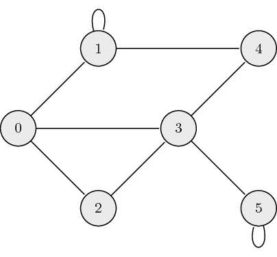
The following is an example of an undirected graph:

The adjacency matrix, \({\bf A}\), for undirected graphs is always symmetric and is defined as:

\[a_{ij} = \begin{cases} 1 \quad \mathrm{if} \ (\mathrm{node}_i, \mathrm{node}_j) \ \textrm{are connected} \\ 0 \quad \mathrm{otherwise} \end{cases},\]

where \(a_{ij}\) is the \((i,j)\) element of \({\bf A}\). The adjacency matrix which describes the example graph above is:

\[ {\bf A} = \begin{bmatrix} 0 & 1 & 1 & 1 & 0 & 0 \\ 1 & 1 & 0 & 0 & 1 & 0 \\ 1 & 0 & 0 & 1 & 0 & 0 \\ 1 & 0 & 1 & 0 & 1 & 1 \\ 0 & 1 & 0 & 1 & 0 & 0 \\ 0 & 0 & 0 & 1 & 0 & 1 \end{bmatrix}.\]

Directed Graphs:

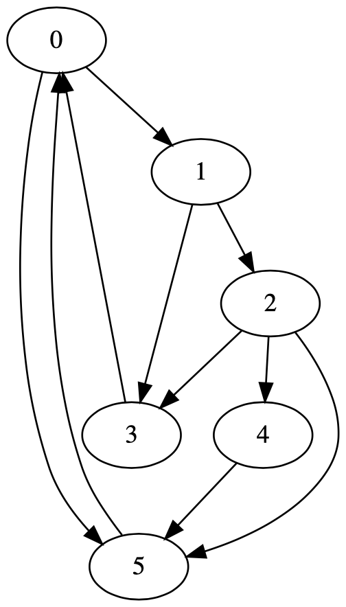
The following is an example of a directed graph:

The adjacency matrix, \({\bf A}\), for directed graphs is defined as:

\[ a_{ij} = \begin{cases} 1 \quad \mathrm{if} \ \mathrm{node}_i \leftarrow \mathrm{node}_j \\ 0 \quad \mathrm{otherwise} \end{cases}, \]

where \(a_{ij}\) is the \((i,j)\) element of \({\bf A}\). This matrix is typically asymmetric, so it is important to adhere to the definition. Note that while we effectively use columns to represent the "from" nodes and rows to represent the "to" nodes, this is not necessarily standard and you may encounter the reverse direction. The adjacency matrix which describes the example graph above is:

\[ {\bf A} = \begin{bmatrix} 0 & 0 & 0 & 1 & 0 & 0 \\ 1 & 1 & 0 & 0 & 0 & 0 \\ 1 & 0 & 0 & 0 & 0 & 0 \\ 0 & 0 & 1 & 0 & 1 & 0 \\ 0 & 1 & 0 & 0 & 0 & 0 \\ 0 & 0 & 0 & 1 & 0 & 1 \end{bmatrix}.\]

Weighted Directed Graphs:

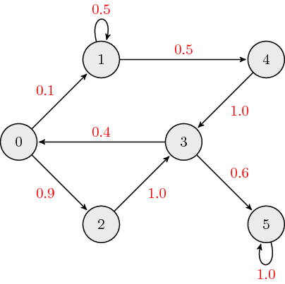
The following is an example of a weighted directed graph:

The adjacency matrix, \({\bf A}\), for weighted directed graphs is defined as:

\[ a_{ij} = \begin{cases} w_{ij} \quad \mathrm{if} \ \mathrm{node}_i \leftarrow \mathrm{node}_j \\ 0 \quad \ \ \mathrm{otherwise} \end{cases}, \]

where \(a_{ij}\) is the \((i,j)\) element of \({\bf A}\), and \(w_{ij}\) is the link weight associated with edge connecting nodes \(i\) and \(j\). The adjacency matrix which describes the example graph above is:

\[ {\bf A} = \begin{bmatrix} 0 & 0 & 0 & 0.4 & 0 & 0 \\ 0.1 & 0.5 & 0 & 0 & 0 & 0 \\ 0.9 & 0 & 0 & 0 & 0 & 0 \\ 0 & 0 & 1.0 & 0 & 1.0 & 0 \\ 0 & 0.5 & 0 & 0 & 0 & 0 \\ 0 & 0 & 0 & 0.6 & 0 & 1.0 \end{bmatrix}.\]

Typically, when we discuss weighted directed graphs it is in the context of transition matrices for Markov chains where the link weights across each column sum to \(1\).

Markov Chain

A Markov chain is a stochastic model where the probability of future (next) state depends only on the most recent (current) state. This memoryless property of a stochastic process is called Markov property. From a probability perspective, the Markov property implies that the conditional probability distribution of the future state (conditioned on both past and current states) depends only on the current state.

The Markov property, more formally can be written as:

\[P(X_{n+1} = x_{n+1} | X_0 = x_0, X_1 = x_1, ..., X_n = x_n) = P(X_{n+1} = x_{n+1} | X_n = x_n)\]

Markov Matrix

A Markov/Transition/Stochastic matrix is a square matrix used to describe the transitions of a Markov chain. Each of its entries is a non-negative real number representing a probability. Based on Markov property, next state vector \({\bf x}_{k+1}\) is obtained by left-multiplying the Markov matrix \({\bf M}\) with the current state vector \({\bf x}_k\).

\[ {\bf x}_{k+1} = {\bf M} {\bf x}_k \]

In this course, unless specifically stated otherwise, we define the transition matrix \({\bf M}\) as a left Markov matrix where each column sums to \(1\). Alternatively, we can say the \(1\text{-}norm\) of each column is \(1\).

Note: Alternative definitions in outside resources may present \({\bf M}\) as a right markov matrix where each row of \({\bf M}\) sums to \(1\) and the next state is obtained by right-multiplying by \({\bf M}\), i.e. \({\bf x}_{k+1}^T = {\bf x}_k^T {\bf M}\).

A steady state vector \({\bf x}^*\) is a probability vector (entries are non-negative and sum to \(1\)) that is unchanged by the operation with the Markov matrix \(M\), i.e.

\[ {\bf M} {\bf x}^* = {\bf x}^* \]

Therefore, the steady state vector \({\bf x}^*\) is an eigenvector corresponding to the eigenvalue \(\lambda=1\) of matrix \({\bf M}\). If there is more than one eigenvector with \(\lambda=1\), then a weighted sum of the corresponding steady state vectors will also be a steady state vector. Therefore, the steady state vector of a Markov chain may not be unique and could depend on the initial state vector.

In summary, repeated multiplication of a state vector \({\bf x}\) from the left by a Markov matrix \({\bf M}\)converges to a vector of eigenvalue \(\lambda=1\). This should remind you of the Power Iteration method. The largest eigenvalue of a Markov matrix by magnitude is always 1.

Markov Chain Example: Weather

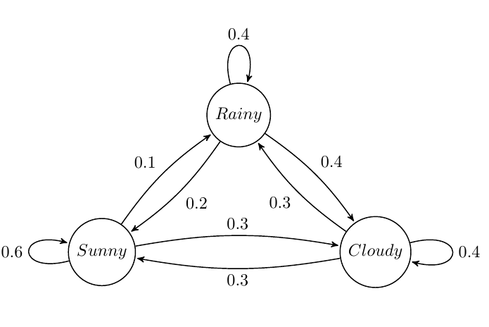
Suppose we want to build a Markov Chain model for weather predicting in UIUC during summer. We observed that:

a sunny day is \(60\%\) likely to be followed by another sunny day, \(10\%\) likely followed by a rainy day and \(30\%\) likely followed by a cloudy day;
a rainy day is \(40\%\) likely to be followed by another rainy day, \(20\%\) likely followed by a sunny day and \(40\%\) likely followed by a cloudy day;
a cloudy day is \(40\%\) likely to be followed by another cloudy day, \(30\%\) likely followed by a rainy day and \(30\%\) likely followed by a sunny day.

The state diagram is shown below:

The Markov matrix is

\[ {\bf M} = \begin{bmatrix} 0.6 & 0.2 & 0.3 \\ 0.1 & 0.4 & 0.3 \\ 0.3 & 0.4 & 0.4 \end{bmatrix}. \]

If the weather on day \(0\) is known to be rainy, then

\[ {\bf x}_0 = \begin{bmatrix} 0 \\ 1 \\ 0 \end{bmatrix}; \]

and we can determine the probability vector for day \(1\) by

\[ {\bf x}_1 = {\bf M} {\bf x}_0. \]

The probability distribution for the weather on day \(n\) is given by

\[ {\bf x}_n = {\bf M}^{n} {\bf x}_0. \]

Markov Chain Example: Page Rank

Page Rank is a straightforward algorithm which was popularized by Google Search to rank webpages. It attempts to model user behavior by assuming a random surfer continuously clicks links at random. So, the importance of a web page is determined by the probability of a random user ending up at that page.

Let the above graph represent websites as nodes and outgoing links as directed eges. First, we create an adjacency matrix.

\[ {\bf A} = \begin{bmatrix} 0 & 0 & 0 & 1 & 0 & 1 \\ 1 & 0 & 0 & 0 & 0 & 0 \\ 0 & 1 & 0 & 0 & 0 & 0 \\ 0 & 1 & 1 & 0 & 0 & 0 \\ 0 & 0 & 1 & 0 & 0 & 0 \\ 1 & 0 & 1 & 0 & 1 & 0 \\ \end{bmatrix} \]

Next, we take the accumulated weight (influence) going into a given page, and redistribute it evenly across each outgoing link. This is a Markov matrix. As before, we can perform repeated iteration on a random state vector until steady-state in order to find what page the user will most likely end up at.

\[ {\bf A} = \begin{bmatrix} 0 & 0 & 0 & 1.0 & 0 & 1.0 \\ 0.5 & 0 & 0 & 0 & 0 & 0 \\ 0 & 0.5 & 0 & 0 & 0 & 0 \\ 0 & 0.5 & 0.33 & 0 & 0 & 0 \\ 0 & 0 & 0.33 & 0 & 0 & 0 \\ 0.5 & 0 & 0.33 & 0 & 1.0 & 0 \\ \end{bmatrix} \]

Sites therefore become "important" if they're linked to by other "important" sites. The intuition roughly follows that if a site \(s\) is linked within another site that is rarely embedded, then the rank of site \(s\) will not increase much. Conversely, if site \(s\) is linked within more popular sites, its rank will increase.

Naive Page Rank: Shortcomings

A weakpoint of this naive implementation of Page Rank is that a unique solution is not guaranteed. Brin-Page (1990s) proposed:

"PageRank can be thought of as a model of user behavior We assume there is a random surfer who is given a web page at random and keeps clicking on links, never hitting "back", but eventually gets bored and starts on another random page."

\[{\bf{M}} = d{\bf{A}} + \frac{1-d}{n}\bf{1} \]

We introduce a constant, or damping factor, \(d\) in order to model the random jump. Let \(n\) be the number of nodes in the graph. Here, a surfer clicks on a link on the current page with probability \(d\) and opens a random page with probability \(1-d\). This model makes all entries of M greater than zero, and guarantees a unique solution.

Review Questions

Given an undirected or directed graph (weighted or unweighted), determine the adjacency matrix for the graph.
What is a transition matrix? Given a graph representing the transitions or a description of the problem, determine the transition matrix.