Optimization
Learning objectives
- Recognize the goal of optimization: finding an approximation of the minimum of a function
- Understand basic optimization approaches
- Set up a problem as an optimization problem
- Understand two methods of 1-D optimization: Golden Section Search and Newton's Method (1D)
- Understand two methods of N-D optimization: Steepest Descent and Newton's Method (N-D)
- Identify challenges in optimization
Optimization: Finding Minima of a Function
The goal of optimization is to find point(s) in a function's domain that minimize the function.
Consider a function \(f:\;S\to \mathbb{R}\), and \(S\subset\mathbb{R}^n\). The point \(\boldsymbol{x}^*\in S\) is called the minimizer or minimum of \(f\) if \(f(\boldsymbol{x}^*)\leq f(\boldsymbol{x}) \, \forall x\in S\).
There are two types of optimization:
- Unconstrained Optimization: find \(\boldsymbol{x}^*\) such that \(f(\boldsymbol{x}^*) = \underset{\boldsymbol{x}}{\mathrm{min}}\hspace{1mm}f(\boldsymbol{x})\)
- Constrained Optimization: find \(\boldsymbol{x}^*\) such that \(f(\boldsymbol{x}^*) = \underset{\boldsymbol{x}}{\mathrm{min}}\hspace{1mm}f(\boldsymbol{x})\)
\(\hspace{2cm} \text{such that: } \boldsymbol{g}(\boldsymbol{x}) = 0 \hspace{5mm} \leftarrow \hspace{5mm} \text{\small ``Equality Constraints"}\) \(\hspace{2cm} \text{and / or: } \boldsymbol{h}(\boldsymbol{x}) \leq 0 \hspace{5mm} \leftarrow \hspace{5mm} \text{\small ``Inequality Constraints"}\)
for some other functions \(\boldsymbol{g}\) and/or \(\boldsymbol{h}\).
Notice that a solution is not guaranteed to exist for an optimization problem if the domain \(S\) is infinite.
For the rest of this topic we try to find the minimizer of a function. Notice that if we want a maximizer \(\boldsymbol{y}^*\) of a function \(\boldsymbol{f}\) such that \(f(\boldsymbol{y}^{*}) = \underset{\boldsymbol{y}}{\mathrm{max}}\hspace{1mm}f(\boldsymbol{y})\), we can instead solve the minimization problem to find the minimizer \(\boldsymbol{x}^*\) where \(\boldsymbol{x}^*\) such that \(f(\boldsymbol{x}^*) = \underset{\boldsymbol{x}}{\mathrm{min}}(\hspace{1mm}-f(\boldsymbol{x}))\).
Example: Calculus problem
Given \(d_1, d_2 \gt 0\), find:
\[\boxed{ \begin{aligned} \underset{\boldsymbol{d \in \mathbb{R}^2}}{\mathrm{max}}\hspace{1mm}f(d_1, d_2) &= d_1 \times d_2 \\ \text{\small such that} \quad g(d_1, d_2) &= 2(d_1+d_2) - 20 \leq 0 \end{aligned} }\]Notice that \(\underset{\boldsymbol{d \in \mathbb{R}^2}}{\mathrm{max}}\hspace{1mm}f(d_1, d_2) = \underset{\boldsymbol{d \in \mathbb{R}^2}}{\mathrm{min}}\hspace{1mm}(-f(d_1, d_2))\), so we can instead solve the following optimization problem:
\[\boxed{ \begin{aligned} \underset{\boldsymbol{d \in \mathbb{R}^2}}{\mathrm{min}}\hspace{1mm}(-f(d_1, d_2)) &= -(d_1 \times d_2) \\ \text{\small such that} \quad g(d_1, d_2) &= 2(d_1+d_2) - 20 \leq 0 \end{aligned} }\]More Details
In fact, this question asked for minimizing maximizing the rectangle area subject to perimeter constraint (20). The red region below gives a demo: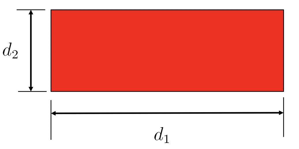
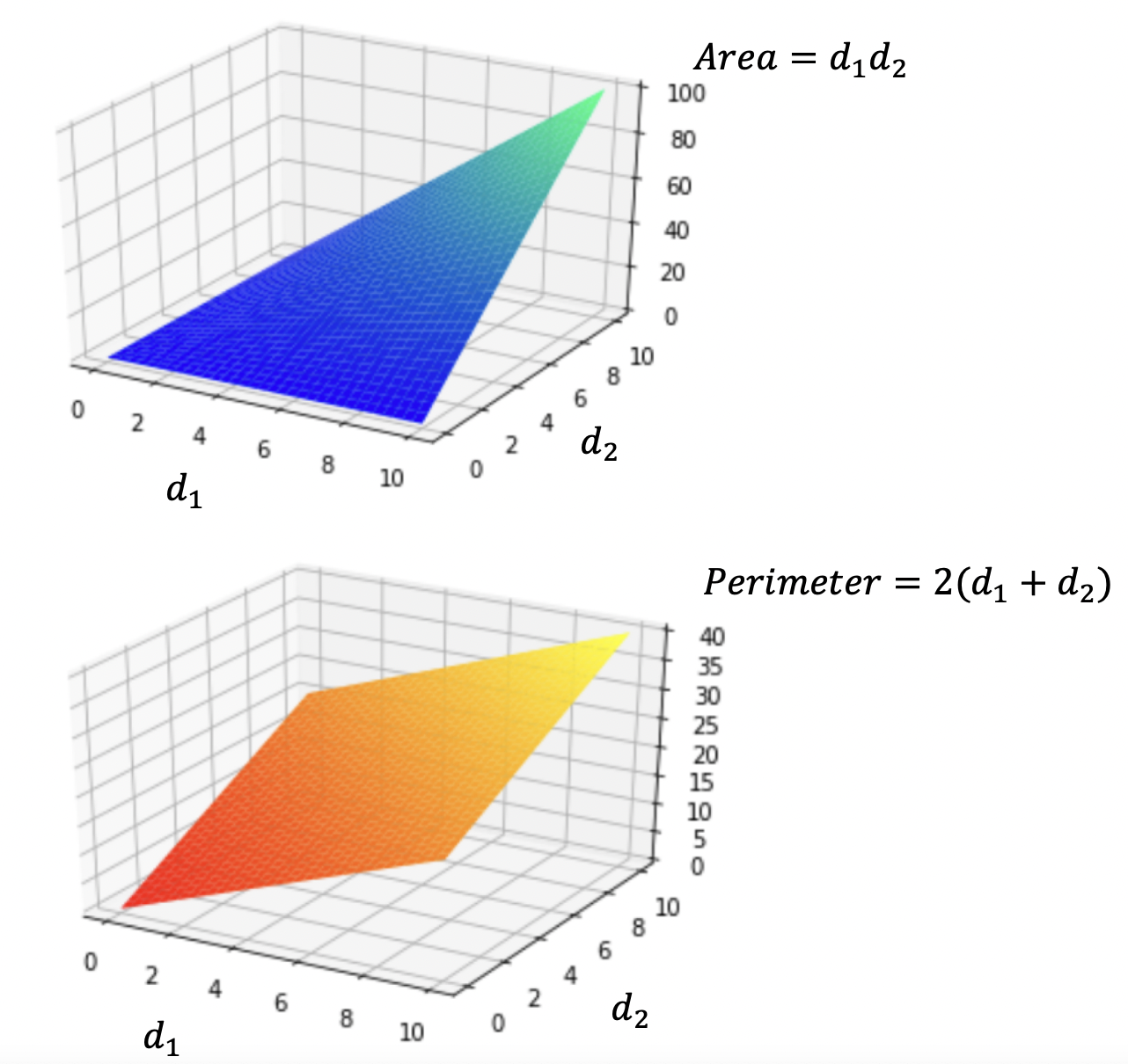
Here's a visualization of the relationship between \(d_1\) and \(d_2\) in terms of area and perimeter:
Local vs. Global Minima
Consider a domain \(S\subset\mathbb{R}^n\), and \(f:S\to\mathbb{R}\).
-
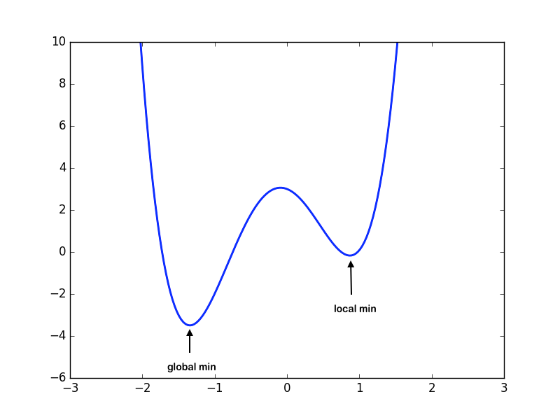
Local Minima: \(\boldsymbol{x}^*\) is a local minimum if \(f(\boldsymbol{x}^*)\leq f(\boldsymbol{x})\) for all feasible \(\boldsymbol{x}\) in some neighborhood of \(\boldsymbol{x}^*\).
-
Global Minima: \(\boldsymbol{x}^*\) is a global minimum if \(f(\boldsymbol{x}^*)\leq f(\boldsymbol{x})\) for all \(\boldsymbol{x}\in S\).
Note that it is easier to find the local minimum than the global minimum. Given a function, finding whether a global minimum exists over the domain is in itself a non-trivial problem. Hence, we will limit ourselves to finding the local minima of the function.
Also, note that a function can always have more than 1 minima.
Two Types of Methods to Resolve 1-Dimensional Optimization Problems
First, let's learn about some techniques to resolve 1-D optimization problems.
Given a nonlinear, continuous and smooth function \(f:\;\mathbb{R}\to \mathbb{R}\) and the optimization problem \(f(\boldsymbol{x}^*) = \underset{\boldsymbol{x \in S}}{\mathrm{min}}\hspace{1mm}f(\boldsymbol{x})\), there are two types of methods which we'll cover in this class:
- Derivative-free methods: Only requiring the evaluation of \(f(\boldsymbol{x})\) on a set of \(x \in S\). In particular, we cover the Golden Section Search method.
- Second-derivative methods: Requiring the evaluation of \(f(\boldsymbol{x})\), \(f'(\boldsymbol{x})\), and \(f''(\boldsymbol{x})\) and on a set of \(x \in S\). In particular, we cover Newton's Method for 1-D.
Criteria for 1-D Local Minima
In the case of 1-D optimization, we need to find the minima of a continuous and smooth function \(f:\;\mathbb{R} \to \mathbb{R}\). Recall from calculus that when \(f'(x^*) = 0\), we get a local maximum if \(f''(x^*) < 0\), and a local minimum if \(f''(x^*) > 0\). (Notice that we cannot conclude anything if \(f''(x^*) = 0\)). We can then tell if a point \(x^* \in S\) is a local minimum (i.e., find \(\boldsymbol{x}^*\) such that \(f(\boldsymbol{x}^*) = \underset{\boldsymbol{x}}{\mathrm{min}}\hspace{1mm}f(\boldsymbol{x})\)) by getting the values of the first and second derivatives. Specifically,
- (First-order) Necessary condition: \(f'(x^*) = 0\)
- (Second-order) Sufficient condition: \(f'(x^*) = 0\) and \(f''(x^*) > 0\).
Example: 1-D Optimization Problem
Consider the function \(f(x) = x^3 - 6x^2 + 9x -6\)
How can we find a local minimum of it?
Answer
The first and second derivatives are as follows: $$f'(x) = 3x^2-12x+9$$ $$f''(x) = 6x-12$$ The critical points are tabulated as:| \({x}\) | \({f'(x)}\) | \({f''(x)}\) | Characteristic |
|---|---|---|---|
| 3 | 0 | \(6\) | Local Minimum |
| 1 | 0 | \(-6\) | Local Maximum |
Example: Find All Stationary Points of a 1-D Function
Consider the function \(f(x) = \frac{x^4}{4} - \frac{x^3}{3} - 11x^2 + 40x\)
Find the stationary points and check the sufficient conditions.
Answer
The gradient vector and the Hessian matrix for \(f\) are as follows: $$f'(x) = \frac{4x^3}{4} - \frac{3x^2}{3} - 22x +40 = x^3 - x^2 - 22x + 40$$ $$f''(x) = 3x^2 - 2x - 22$$ Solve for \(f'(x) = 0\) gives three possible solutions, namely \(x_1 = -5, x_2 = 2, \text{and }x_3 = 4\).Now, observe that:
(1) \(f''(x_1) = 3 \times (-5)^2 - 2 \times (-5) - 22 \gt 0\) \(\rightarrow\) \(\bf{x_1 = -5}\) is a local \(\textbf{minimum}\).
(2) \(f''(x_2) = 3 \times (2)^2 - 2 \times 2 - 22 \lt 0\) \(\rightarrow\) \(\bf{x_2 = 2}\) is a local \(\textbf{maximum}\).
(3) \(f''(x_3) = 3 \times (4)^2 - 2 \times 4 - 22 \gt 0\) \(\rightarrow\) \(\bf{x_3 = 4}\) is a local \(\textbf{minimum}\).
Unimodal Functions
Let us consider a special family of functions that makes the optimization task easier:
A function \(f:\mathbb{R}\to \mathbb{R}\) is unimodal on an interval \([a,b]\) if this function has a unique (global) minimum on that interval \([a,b]\)
More rigidly, a 1-dimensional function \(f: S\to\mathbb{R}\), is said to be unimodal on an interval \([a,b]\) if there is a unique \(\bf{x}^* \in [a, b]\) such that \(f(\bf{x}^*)\) is the minimum in \([a, b]\), and that for all \(x_1, x_2 \in [a, b]\) where \(x_1 \lt x_2\), the following two properties hold:
\[x_2 < x^*\Rightarrow f(x_1)>f(x_2)\] \[x^* < x_1\Rightarrow f(x_1)<f(x_2)\]Some examples of unimodal functions on an interval:
-
\(f(x) = x^2\) is unimodal on the interval \([-1,1]\)
-
\(f(x) = \begin{cases} x, \text{ for } x \geq 0, \\ 0, \text{ for } x < 0 \end{cases}\) is not unimodal on \([-1,1]\) because the global minimum is not unique. This is an example of a convex function that is not unimodal.
-
\(f(x) = \begin{cases} x, \text{ for } x > 0, \\ -100, \text{ for } x = 0,\\ 0 \text{ for } x < 0\end{cases}\) is not unimodal on \([-1,1]\). It has a unique minimum at \(x=0\) but does not steadily decrease(i.e., monotonically decrease) as you move from \(-1\) to \(0\).
-
\(f(x) = cos(x)\) is not unimodal on the interval \([-\pi/2, 2\pi]\) because it increases on \([-\pi/2, 0]\).
In order to simplify, we will consider our objective function to be unimodal as it guarantees us a unique solution to the minimization problem.
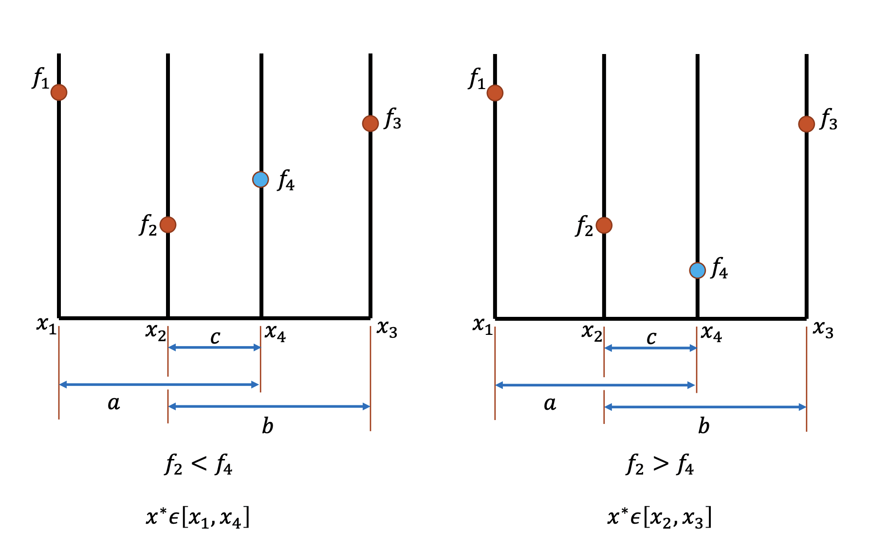
Notice that a given a unimodal function \(f\) and a domain \([a, b]\), we can partition \([a, b]\) into \([x_1, x_2, x_4, x_3]\), where \(x_1 = a, x_3 = b\) and \(x_2 - x_1 = x_4 - x_2 = x_3 - x_4\). Then we can easily verify that if \(f_2 = f(x_2) \lt f(x_4) = f_4\), the minimizer \(x^* \in [x_1, x_4]\). Similarly, if \(f_2 = f(x_2) \gt f(x_4) = f_4\), the minimizer \(x^* \in [x_2, x_3]\). Therefore, we can apply this "partition" process on the smaller interval recursively until it converges to the minimum. Notice that this approach is similar with the binary search method in root finding. A demo of this idea is shown in the graph below:
However, notice that such method would in general require 2 new function evaluations per iteration. Lets see how Golden Section Search can refine this algorithm to require only one function evaluation per step.
Golden Section Search (1-D)
Inspired by the algorithm above, we define an interval reduction method for finding the minimum of a function. As in bisection (for root finding) where we reduce the interval such that the reduced interval always contains the root, in Golden Section Search we reduce our interval such that it always has a unique minimizer in our domain.
Algorithm to find the minima of \(f: [a, b] \to \mathbb{R}\):
Our goal is to introduce "interior" points \(x_1\) and \(x_2\), and reduce the domain to \([x_1, x_2]\) such that:
- If \(f(x_1) > f(x_2)\) our new interval would be \([x_1, b]\)
- If \(f(x_1) \leq f(x_2)\) our new interval would be \([a, x_2]\)
Since we do not want two function evaluations per step, we need to ensure that in the next step:
- If the input domain is \([a, x_2]\), reuse \(x_1\) as one of the 2 new "interior" points, since it lies between \([a, x_2]\), and \(f(x_1)\) has already been evaluated.
- Similarly, f the input domain is \([x_1, b]\), reuse \(x_2\) as one of the 2 new "interior" points, since it lies between \([x_1, b]\), and \(f(x_2)\) has already been evaluated.
Set \(h_0 = b - a\) and \(h_1 = b - x_1 = x_2 - a\).
Since we want to make sure that the intervals to be examined "shrinks" at a consistent rate, we need a constant \(\tau\) such that \(h_1 = \tau h_0\) (or in general \(h_{k+1} = \tau h_k\) for all \(k \in \mathbb{N}\)).
Since we want to "reuse" either \(x_1\) or \(x_2\), it must hold that \(\tau h_1 = (1 - \tau)h_0\) (You can check it's true using the demo figure above). Subsitutue \(h_1\) by \(\tau h_0\), we get:
\[\tau \tau h_0 = (1 - \tau)h_0\] \[\tau ^2 = (1 - \tau)\] \[\bf{\tau} = \frac{\sqrt{5}-1}{2} \approx \textbf{0.618}\]Notice that:
\[x_1 = a + (1-\tau)(b-a)\] \[x_2 = a + \tau(b-a)\]As the interval gets reduced by a fixed factor each time, it can be observed that the method is linearly convergent:
\[\lim_{k \to \infty} \frac{\vert e_{k+1} \vert}{\vert e_k \vert} = \tau \approx 0.618\]The number \(\frac{\sqrt{5}-1}{2}\) is the inverse of the "Golden-Ratio" and hence this algorithm is named Golden Section Search.
In golden section search, we do not need to evaluate any derivatives of \(f(x)\). At each iteration we need \(f(x_1)\) and \(f(x_2)\), one of \(x_1\) or \(x_2\) will be the same as the previous iteration, so it only requires 1 additional function evaluation per iteration (after the first iteration).
Example: Golden Section Search "Bracket Length"
Consider running Golden Section search on a function that is unimodal. If golden section search is started with an initial bracket of \([-10, 10]\), what is the length of the new bracket after 1 iteration?
Answer
$$(10 - (-10)) \times \tau \approx 12.36$$Newton's Method (1-D)
Using Taylor Expansion, we can approximate the function \(f\) with a quadratic function about \(x_0\):
\[f(x) \approx f(x_0) + f'(x_0)(x - x_0) + \frac{1}{2}f''(x_0)(x - x_0)^2\]And we want to find the minimum of the quadratic function using the first-order necessary condition:
\[f'(x) = 0 \Rightarrow f'(x_0) + f''(x_0)(x - x_0) = 0\] \[h = (x - x_0) \Rightarrow h = \frac{-f'(x_0)}{f''(x_0)}\]Note that this is the same as the step for the Newton's method to solve the nonlinear equation \(f'(x) = 0\)
We know that in order to find a local minimum we need to find the root of the derivative of the function. Inspired from Newton's method for root-finding we define our iterative scheme as follows:
\[\bf{x_0} = \textbf{starting guess}\] \[\bf{x_{k+1}} = x_k - \frac{f'(x_k)}{f''(x_k)}\]The method typically converges quadratically, provided that \(x_k\) is sufficiently close to the local minimum. In other words, Newton's method has local convergence, and may fail to converge, or converge to a maximum or point of inflection.
For Newton's method for optimization in 1-D, we evaluate \(f'(x_k)\) and \(f''(x_k)\), so it requires 2 function evaluations per iteration.
Example: Newton's Method for 1-D
Consider the function \(f(x) = 4x^3 + 2x^2 + 5x + 40\). If we use the initial guess \(x_0 = 2\), what would be the value of \(x\) after one iteration of the Newton's method?
Answer
To apply the first step Newton's method for optimization, we use the iterative formula to get: \[ x_1 = x_0 - \frac{f'(x_0)}{f''(x_0)} \] Given the function \( f(x) = 4x^3 + 2x^2 + 5x + 40 \), its first derivative \( f'(x) \) is: \[ f'(x_0) = 12x^2 + 4x + 5 \] Hence \[ f'(2) = 12(2)^2 + 4(2) + 5 = 12(4) + 8 + 5 = 48 + 8 + 5 = 61 \] And its second derivative \( f''(x) \) is: \[ f''(x) = 24x + 4 \] Hence \[ f''(x_0) = 24(2) + 4 = 48 + 4 = 52 \] Finally, apply Newton's method formula: \[ x_1 = 2 - \frac{61}{52} \approx 0.827 \]Definiton of Gradient and Hessian Matrix
Now let us revise some key concepts useful in solving N-dimensional optimization problems:
Given \(f:\mathbb{R}^n\to \mathbb{R}\), we define the gradient function \(\nabla f: \mathbb{R}^n\to\mathbb{R}^n\) as:
\[\nabla f(\boldsymbol{x}) = \begin{bmatrix} \dfrac{\partial f}{\partial x_1} \\ \dfrac{\partial f}{\partial x_2} \\ \vdots \\ \dfrac{\partial f}{\partial x_n} \\ \end{bmatrix}\]Given \(f:\mathbb{R}^n\to \mathbb{R}\), we define the Hessian matrix \({\bf H}_f: \mathbb{R}^n\to\mathbb{R}^{n\times n}\) as:
\[{\bf H}_f(\boldsymbol{x}) = \begin{bmatrix} \dfrac{\partial^2 f}{\partial x_1^2} & \dfrac{\partial^2 f}{\partial x_1 \partial x_2} & \ldots & \dfrac{\partial^2 f}{\partial x_1 \partial x_n} \\ \dfrac{\partial^2 f}{\partial x_2 \partial x_1} & \dfrac{\partial^2 f}{\partial x_2^2} & \ldots & \dfrac{\partial^2 f}{\partial x_2 \partial x_n} \\ \vdots & \vdots & \ddots & \vdots \\ \dfrac{\partial^2 f}{\partial x_n \partial x_1} & \dfrac{\partial^2 f}{\partial x_n \partial x_2} & \ldots & \dfrac{\partial^2 f}{\partial x_n^2} \end{bmatrix}\]Two Types of Methods to Resolve N-Dimensional Optimization Problems
Given a nonlinear, continuous and smooth function \(f:\;\mathbb{R}^n\to \mathbb{R}\) and the optimization problem \(f(\boldsymbol{x}^*) = \underset{\boldsymbol{x \in S}}{\mathrm{min}}\hspace{1mm}f(\boldsymbol{x})\), there are two types of methods which we'll cover in this class:
- Gradient (first-derivative) methods: Requiring the evaluation of \(f(\boldsymbol{x})\) and \(\nabla f(\boldsymbol{x})\) on a set of \(x \in S\). In particular, we cover the Steepest Descent method.
- Hessian (second-derivative) methods: Requiring the evaluation of \(f(\boldsymbol{x})\), \(\nabla f(\boldsymbol{x})\), and \({\nabla}^2 f(\boldsymbol{x})\) and on a set of \(x \in S\). In particular, we cover Newton's Method for N-D.
where:
\[\boldsymbol{x} = \begin{bmatrix}x_1, x_2, \ldots, x_n\end{bmatrix}\] \[f(\boldsymbol{x}) = f(\begin{bmatrix}x_1, x_2, \ldots, x_n\end{bmatrix})\] \[\nabla f(\boldsymbol{x}) = \text{\small gradient} (x) = \begin{bmatrix} \dfrac{\partial f}{\partial x_1} \\ \dfrac{\partial f}{\partial x_2} \\ \vdots \\ \dfrac{\partial f}{\partial x_n} \\ \end{bmatrix}\] \[{\nabla}^2 f(\boldsymbol{x}) = {\bf H}_f(\boldsymbol{x}) = \begin{bmatrix} \dfrac{\partial^2 f}{\partial x_1^2} & \dfrac{\partial^2 f}{\partial x_1 \partial x_2} & \ldots & \dfrac{\partial^2 f}{\partial x_1 \partial x_n} \\ \dfrac{\partial^2 f}{\partial x_2 \partial x_1} & \dfrac{\partial^2 f}{\partial x_2^2} & \ldots & \dfrac{\partial^2 f}{\partial x_2 \partial x_n} \\ \vdots & \vdots & \ddots & \vdots \\ \dfrac{\partial^2 f}{\partial x_n \partial x_1} & \dfrac{\partial^2 f}{\partial x_n \partial x_2} & \ldots & \dfrac{\partial^2 f}{\partial x_n^2} \end{bmatrix}\]Criteria for N-D Local Minima
In the case of n-dimensional optimization, we need to find the minima of a continuous and smooth function \(f:\;\mathbb{R}^n \to \mathbb{R}\). We can tell if a point \(x^* \in S\) is a local minimum by considering the values of the gradients and Hessians. Notice that N-D gradient is equivalent to 1-D derivative, and the Hessian matrix has following properties at points of zero gradient:
| \( H_f(x^*) \) | Eigenvalues of \( H_f(x^*) \) | Critical Point \( x^* \) |
|---|---|---|
| Positive Definite | All Positive | Minimizer |
| Negative Definite | All Negative | Maximizer |
| Indefinite | Indefinite | Saddle Point |
Therefore, below are the conditions to find \(\boldsymbol{x}^*\) such that \(f(\boldsymbol{x}^*) = \underset{\boldsymbol{x}}{\mathrm{min}}\hspace{1mm}f(\boldsymbol{x})\):
- Necessary condition: the gradient \(\nabla f(\boldsymbol{x}^*) = \boldsymbol{0}\)
- Sufficient condition: the gradient \(\nabla f(\boldsymbol{x}^*) = \boldsymbol{0}\) and the Hessian matrix \(H_f(\boldsymbol{x^*})\) is positive definite.
Example: Find All Stationary Points of a N-D Function
Consider the function
\[f(x_1, x_2) = 2x_1^3 + 4x_2^2 + 2x_2 - 24x_1\]Find the stationary points and check the sufficient conditions.
Answer
The gradient is as follows: \[ \nabla f(\boldsymbol{x}) = \text{\small gradient} (x) = \begin{bmatrix} 6x_1^2 - 24 \\ 8x_2 + 2 \\ \end{bmatrix} \] Solving for \(\nabla f = 0 \text{ gives }6x_1^2 - 24 = 0\text{ and }8x_2 + 2 = 0\text{, so }x_1 = \pm 2 \text{ and } x_2 = -0.25\).The Hessian matrix is as follows: \[ {\bf H}_f(\boldsymbol{x}) = \begin{bmatrix} 12x_1 & 0\\ 0 & 8 \\ \end{bmatrix} \] \(\textbf{Situation 1:}\)
\[ x^* = \begin{bmatrix} 2 \\ -0.25 \\ \end{bmatrix} \rightarrow {\bf H}_f = \begin{bmatrix} 24 & 0 \\ 0 & 8 \\ \end{bmatrix} \] The Hessian is positive definite (contains only positive eigenvalues), so that \(x^* = \begin{bmatrix} 2 \\ -0.25 \\ \end{bmatrix}\) is a \(\textbf{local minimum}\).
\(\textbf{Situation 2:}\)
\[ x^* = \begin{bmatrix} -2 \\ -0.25 \\ \end{bmatrix} \rightarrow {\bf H}_f = \begin{bmatrix} -24 & 0 \\ 0 & 8 \\ \end{bmatrix} \] The Hessian is indefinite, so that \(x^* = \begin{bmatrix} 2 \\ -0.25 \\ \end{bmatrix}\) is a \(\textbf{saddle point}\).
Steepest Descent (N-D)
The negative of the gradient of a differentiable function \(f: \mathbb{R}^n\to\mathbb{R}\) points downhill (i.e. towards points in the domain having lower values). In other words, given a function \(f:\mathbb{R}^n\to \mathbb{R}\) at a point \(\bf{x}\), the function will decrease its value in the direction of "steepest descent" \(\bf{-\nabla f}\).
This hints us to move in the direction of \(-\nabla f\) while searching for the minimum until we reach the point where \(\nabla f(\boldsymbol{x}) = \boldsymbol{0}\). Rigidly, for an arbitrary point \(\boldsymbol{x}\), the direction ‘'\(-\nabla f(\boldsymbol{x})\)'' is called the direction of steepest descent. If we resolve this problem in an iterative approach, then in the \(\bf{k^{th}}\) iteration, we define the current steepest descent direction for the current approximation \(\boldsymbol{x_k}\):
\[\boldsymbol{s_{k}} = -\nabla f(\boldsymbol{x_k})\]We know the direction we need to move to approach the minimum but we still do not know the distance we need to move in order to approach the minimum. We need to perform a "line search" among the steepest descent direction. If \(\boldsymbol{x_k}\) was our earlier point then we select the next guess by moving it in the direction of the negative gradient:
\[\boldsymbol{x_{k+1}} = \boldsymbol{x_k} + \alpha(-\nabla f(\boldsymbol{x_k})).\]The next problem would be to find the \(\boldsymbol{\alpha}\), and we use the 1-dimensional optimization algorithms to find the required \(\boldsymbol{\alpha}\). With current \(\boldsymbol{x_k}\), the following equation defines \(\boldsymbol{\alpha_k}\), the optimal choice of \(\boldsymbol{\alpha}\) that brings \(\boldsymbol{x_{k+1}}\) to the minimal point in the line search:
\[\boldsymbol{\alpha_k} = \underset{\alpha}{\mathrm{argmin}}\left( f\left(\boldsymbol{x_k} + \alpha \boldsymbol{s_k}\right)\right)\]Hence in each iteration we calculate:
\[\bf{x_{k+1} = x_k + \alpha _k s_k}\]The Steepest Descent algorithm can be formalized as:
- Initial Guess: \(\bf{x_0}\)
- Evaluate Steepest Descent: \(\bf{s_k = -\nabla f(x_k)}\)
- Perform a line search to obtain \(\alpha _k\) (for example, Golden Section Search): \(\alpha_k = \underset{\alpha}{\mathrm{argmin}} f(\bf{x_k} + \alpha \bf{s_k})\)
- Update: \(\bf{x_{k+1} = x_k + \alpha _k s_k}\)
Generally, the steepest descent method converges linearly.
To translate this algorithm to Python:
import numpy.linalg as la
import scipy.optimize as opt
import numpy as np

def obj_func(alpha, x, s):
    # code for computing the objective function at (x+alpha*s)
    return f_of_x_plus_alpha_s

def gradient(x):
    # code for computing gradient
    return grad_x

def steepest_descent(x_init):
    x_new = x_init
    x_prev = np.random.randn(x_init.shape[0])
    while(la.norm(x_prev - x_new) > 1e-6):
        x_prev = x_new
        s = -gradient(x_prev)
        alpha = opt.minimize_scalar(obj_func, args=(x_prev, s)).x
        x_new = x_prev + alpha*s

    return x_new
Side Note: Observe that \(x_{k+1} = \bf{x_k} - \alpha _k \nabla f(x_k)\), so \(\frac{dx_{k+1}}{d\alpha} = -\nabla f(x_k)\). Since \(\alpha_k = \underset{\alpha}{\mathrm{argmin}} f(\bf{x_k} + \alpha \bf{s_k})\), one necessary condition of the line search is \(\frac{df}{d\alpha} = 0\). Then according to chain rule:
\[\frac{df}{d\alpha} = \frac{df}{dx_{k+1}}\frac{dx_{k+1}}{d\alpha} = -\nabla f(x_{k+1})^T \nabla f(x_k) = 0\]So \(\nabla f(x_{k+1})\) is orthogonal to \(\nabla f(x_k)\).
Example: Steepest Descent Direction
Consider the function \(f(x_1, x_2) = 10(x_1)^3 - (x_2)^2 + x_1 - 1\). What is the steepest descent direction at the starting guess \(x_1 = 2, x_2 = 2\)?
Answer
\[ -\bf{\nabla} f(\bf{\begin{bmatrix} x_1 \\ x_2 \\ \end{bmatrix}}) = - \begin{bmatrix} 30x_1^2 + 1 \\ -2x_2 \\ \end{bmatrix} \] \[ -\bf{\nabla} f(\bf{\begin{bmatrix} 2 \\ 2 \\ \end{bmatrix}}) = - \begin{bmatrix} 30 \times 4 + 1 \\ -2 \times 2 \\ \end{bmatrix} = \bf{\begin{bmatrix} -121 \\ 4 \\ \end{bmatrix}} \]Example: Steepest Descent Iteration
Consider the function \(f(x_1, x_2) = (x_1 - 1)^2 + (x_2 - 1)^2\). What is the steepest descent direction at the starting guess \(y_0 = [3, 3]^T\)? What will \(y_1\) be if we choose \(\alpha_0 = 1\)?
Answer
\[ y_1 = y_0 - \alpha_0 \nabla f(x_0) \] \[ -\bf{\nabla} f(x) = - \begin{bmatrix} 2(y_1 - 1) \\ 2(y_2 - 1) \\ \end{bmatrix} = \bf{\begin{bmatrix} -4 \\ -4 \\ \end{bmatrix}} \] \[ y_1 = - \begin{bmatrix} 3 \\ 3 \\ \end{bmatrix} + 1 \times \bf{\begin{bmatrix} -4 \\ -4 \\ \end{bmatrix}} = \bf{\begin{bmatrix} -1 \\ -1 \\ \end{bmatrix}} \]Example: Step Size
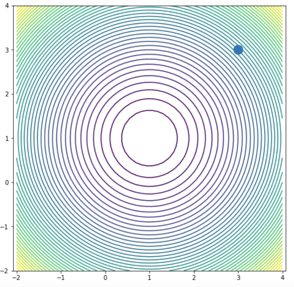
Consider the same function \(f(x_1, x_2) = (x_1 - 1)^2 + (x_2 - 1)^2\) and the initial guess \(y_0 = [3, 3]^T\). You're now given a contour map visualization of this function. What is the ideal choice of \(\alpha\)?
Answer
From the contour map, observe that \(f\) has a local minimum at \( \bf{\begin{bmatrix} 1 \\ 1 \\ \end{bmatrix}} \). Recall from the previous question that \[ \bf{\nabla} f(\bf{y_0}) = \bf{\begin{bmatrix} -4 \\ -4 \\ \end{bmatrix}} \]It is clear that with \(\alpha = 0.5\), \[ \bf{y_1} = \begin{bmatrix} 3 \\ 3 \\ \end{bmatrix} - 0.5 \times \begin{bmatrix} 4 \\ 4 \\ \end{bmatrix} = \bf{\begin{bmatrix} 1 \\ 1 \\ \end{bmatrix}} \] So with \(\bf{\alpha = 0.5}\), Steepest Descent algorithm converge to the minimum after exactly 1 iteration.
Newton's Method (N-D)
Newton's Method in \(n\) dimensions is similar to Newton's method for root finding in \(n\) dimensions, except we just replace the \(n\)-dimensional function by the gradient and the Jacobian matrix by the Hessian matrix. We can arrive at the result by considering the Taylor expansion of the function.
\[f(\boldsymbol{x}+s) \approx f(\boldsymbol{x}) + \nabla f(\boldsymbol{x})^Ts + \frac{1}{2}s^T {\bf H}_f(\boldsymbol{x})s = \hat{f}(s)\]We solve for \(\nabla \hat{f}(\boldsymbol{s}) = \boldsymbol{0}\) for \(\boldsymbol{s}\). Hence the equation can be translated as:
\[\nabla f(\boldsymbol{x}) + \frac{1}{2}\cdot 2 {\bf H}_f(\boldsymbol{x})s = 0\] \[{\bf H}_f(\boldsymbol{x})\boldsymbol{s} = -\nabla f(\boldsymbol{x})\]Which becomes a system of linear equations where we need to solve for the Newton step \(\boldsymbol{s}\).
The steps of the N-Dimensional Newton's Method for optimization can be formally described as follows:
- Initial Guess: \(\boldsymbol{x_0}\)
- Solve: \({\bf H}_f(\boldsymbol{x_k})\boldsymbol{s_k} = -\nabla f(\boldsymbol{x_k})\)
- Update: \(\bf{x_{k+1}} = \bf{x_k} + \bf{s_k}\)
Note that the Hessian is related to the curvature and therefore contains the information about how large the step should be.
Some properties of this algorithm:
- Quadratic convergence in normal circumstances.
- Need second derivatives L.
- Local convergence (requires start guess to be close to solution).
- Works poorly when Hessian is nearly indefinite.
- Cost per iteration: \(O(n^3)\).
This algorithm can be expressed as a Python function as follows:
import numpy as np
import numpy.linalg as la

def hessian(x):
    # Computes the hessian matrix corresponding the given objective function
    return hessian_matrix_at_x

def gradient(x):
    # Computes the gradient vector corresponding the given objective function
    return gradient_vector_at_x

def newtons_method(x_init):
    x_new = x_init
    x_prev = np.random.randn(x_init.shape[0])
    while(la.norm(x_prev-x_new)>1e-6):
        x_prev = x_new
        s = -la.solve(hessian(x_prev), gradient(x_prev))
        x_new = x_prev + s
    return x_new
Example: One Step of Newton's Method for N-D Optimization
To find a minimum of the function \(f(x, y) = 3x^2 +2y^2\), what is the expression for one step of Newton's method?
Answer
The gradient of \( f(x, y) \) is given by: \[ \nabla f(x, y) = \begin{bmatrix} \frac{\partial f}{\partial x} \\ \frac{\partial f}{\partial y} \end{bmatrix} \] And the Hessian matrix of \( f(x, y) \) is given by: \[ H_f(x, y) = \begin{bmatrix} \frac{\partial^2 f}{\partial x^2} & \frac{\partial^2 f}{\partial x \partial y} \\ \frac{\partial^2 f}{\partial y \partial x} & \frac{\partial^2 f}{\partial y^2} \end{bmatrix} \] The solving step of Newton's algorithm of N-D optimization is: \[ H*f(x_k, y_k)\boldsymbol{s_k} = -\nabla f(x*{k}, y\_{k})\] This is mathematically equivalent to: \[{\bf{s_k}} = - H_f(x_k, y_k)^{-1} \nabla f(x_k, y_k) \] Therefore, the update step of Newton's algorithm of N-D optimization is: \[ \begin{bmatrix} x*{k+1} \\ y*{k+1} \end{bmatrix} = \begin{bmatrix} x_k \\ y_k \end{bmatrix} - H_f(x_k, y_k)^{-1} \nabla f(x_k, y_k) \] Given the function \( f(x, y) = 3x^2 + 2y^2 \), its gradient \( \nabla f(x_k, y_k) \) and Hessian matrix \( H_f(x_k, y_k) \) are: \[ \nabla f(x_k, y_k) = \begin{bmatrix} \frac{\partial f}{\partial x_k} \\ \frac{\partial f}{\partial y_k} \end{bmatrix} = \begin{bmatrix} 6x_k \\ 4y_k \end{bmatrix} \] \[ H_f(x_k, y_k) = \begin{bmatrix} \frac{\partial^2 f}{\partial {x_k}^2} & \frac{\partial^2 f}{\partial x_k \partial y_k} \\ \frac{\partial^2 f}{\partial y_k \partial x_k} & \frac{\partial^2 f}{\partial {y_k}^2} \end{bmatrix} = \begin{bmatrix} 6 & 0 \\ 0 & 4 \end{bmatrix} \] So the answer is: \[ \begin{bmatrix} x*{k+1} \\ y*{k+1} \end{bmatrix} = \begin{bmatrix} x_k \\ y_k \end{bmatrix} - {\begin{bmatrix} 6 & 0 \\ 0 & 4 \end{bmatrix}}^{-1} \begin{bmatrix} 6x_k \\ 4y_k \end{bmatrix} \]Example: Convergence of Newton's Method for N-D Optimization
When using the Newton's Method to find the minimizer of the function \(f(x, y) = 0.5x^2 +2.5y^2\), estimate the number of iterations it would take for convergence?
Answer
Answer: \(\textbf{1}\).Reason: Notice that Newton's Method for N-D Optimization is derived from Taylor series truncated after quadratic terms (i.e,.\(\frac{1}{2}s^T {\bf H}\_f(\boldsymbol{x})s\)). This means that it is accurate for quadratic functions.
Review Questions
- What are the necessary and sufficient conditions for a point to be a local minimum in one dimension?
- What are the necessary and sufficient conditions for a point to be a local minimum in \({n}\) dimensions?
- How do you classify extrema as minima, maxima, or saddle points?
- What is the difference between a local and a global minimum?
- What does it mean for a function to be unimodal?
- What special attribute does a function need to have for golden section search to find a minimum?
- Run one iteration of golden section search.
- Calculate the gradient of a function (function has many inputs, one output)
- Calculate the Jacobian of a function (function has many inputs, many outputs).
- Calculate the Hessian of a function.
- Find the search direction in steepest/gradient descent.
- Why must you perform a line search each step of gradient descent?
- Run one step of Newton's method in one dimension.
- Run one step of Newton's method in \({n}\) dimensions.
- When does Newton's method fail to converge to a minimum?
- What operations do you need to perform each iteration of golden section search?
- What operations do you need to perform each iteration of Newton's method in one dimension?
- What operations do you need to perform each iteration of Newton's method in \({n}\) dimensions?
- What is the convergence rate of Newton's method?